Following on from our Tech Tips focusing on Microsoft Outlook, Microsoft Word, OneDrive for Business and Windows 10 this week we cover Microsoft Excel, but don't worry, you won't find a pivot table in sight!

In this round of Tech Tips we cover: 

• Combine Worksheets
• Add a message to a cell
• Remove duplicate data 
• Highlight Duplicate Values
• Insert a bullet point
• Format painter

Combine Worksheets

Imagine this, you receive a file from a colleague or supplier that has 12 different worksheets for 12 months of data, how can you combine them to make it simpler to use?

In this case, the best solution is to combine all of those worksheets using the “Consolidate” option, and here are the steps for this:

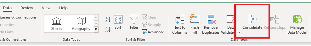
• Add a new worksheet in the workbook and then go to Data Tab ➜ Data Tools ➜ Consolidate.

• You will then see a popup, which is the Consolidate window, from here click on the up arrow in the Reference cell to add the range from the first worksheet that you wish to include in the combined sheet
• click on the Add button.
• Once this is done, you then need to add references from all of the remaining the worksheets using the above step.

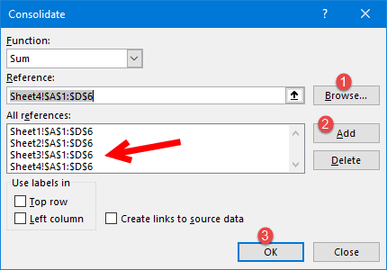
• Once you have all 12 worksheets added click OK 
• This will then create the combined worksheet and you are ready to go with your combined data.

Add a message to a cell

With this tip, let’s say you need to add a specific message to a cell, like “Don’t delete the value”, “enter your name” or something like that.

To do this you can use Data Validation tools to add message for a particular cell so that when a user clicks on the cell they see that message. Here are the steps:

• First, select the cell for which you want to add a message.
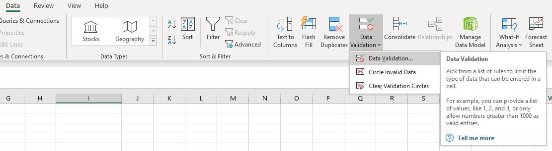
• After that, go to the Data Tab ➜ Data Tools ➜ Data Validation ➜ Data Validation.

• In the data validation window, go to the Input Message tab.

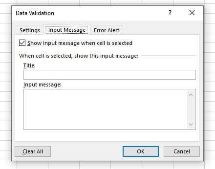
• Enter title, message, and make sure to tick mark Show input message when the cell is selected.

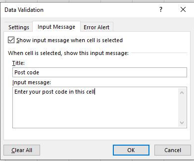
•  Click OK

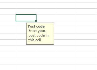
• You will be taken back to the sheet where you can now see your message displayed.  When you click away from the cell the message disappears.

Remove duplicate Data

Sometimes you need to remove duplicate data to simplify a worksheet. For instance, you may have a list of multiple products from the same supplier in your inventory for instance and only want to see the number of suppliers you have. In situations like this, removing the duplicates comes in quite handy.

To remove your duplicates follow these steps:

• Highlight the row or column that you want to remove duplicates of
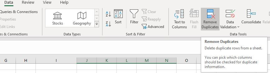
• go to the Data tab and select Remove Duplicates

• A pop-up will appear to confirm which data you want to work with

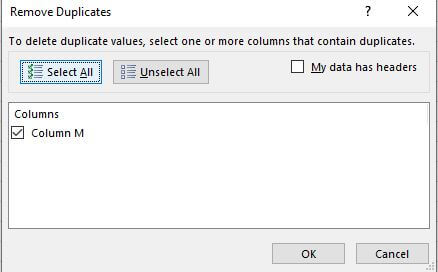
• Select the row or column you want to remove duplicates from and then click on OK
• Excel then removes the duplicates from your chosen area.

Highlight Duplicate Values

Or maybe you would prefer to just highlight duplicate values in a worksheet, here are the steps you need to follow to do this:

• Select the range of where you want to highlight the duplicate values
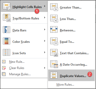
• Go to the Home Tab ➜ Styles ➜ Highlight Cells Rule ➜ Duplicate Values

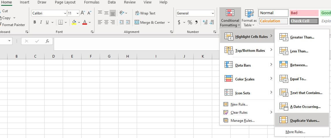
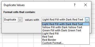
• Now from the dialog box, select the colour to use and click OK.

• Once you click OK, all the duplicate values will be highlighted with your chosen formatting.

Add a bullet point

The easiest way to insert bullet point in Excel is by using custom formatting and here are the steps for this:

1. Press the Ctrl button and the 1 key at the same time (Ctrl + 1) to bring up the Format Cell dialogue box.
2. Under the number tab, select Custom.
3. In the Type: input bar copy the below text and paste it in:

● General;● General;● General;● General

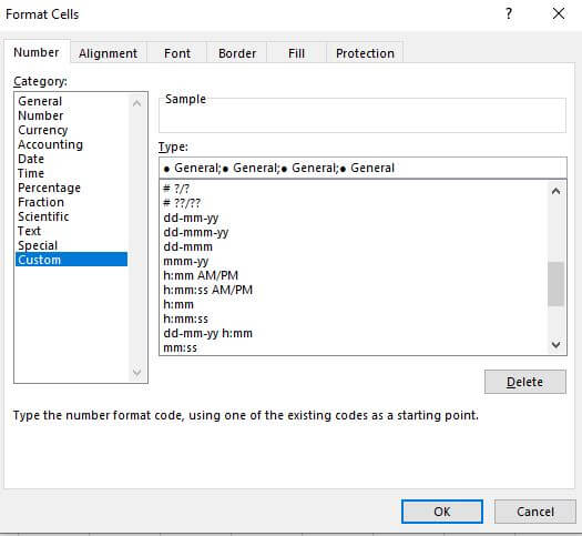
• Click OK.

Now, whenever you enter a value in the cell Excel will add a bullet before that.

Format painter

Format painter allows you to copy and paste formatting from one section to another, say you would like to turn multiple cells into the above bullet point style or you have another set of data that would like to copy the formatting for (Font, Cell Color, Bold, Border, etc.)

Here is how you can do it:

• Select the range you would like to duplicate the format of
• Go to the Home Tab ➜ Clipboard and then click on Format Painter

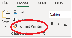
• Highlight the cells you then want to apply the formatting to and they will change to your preferred formatting, just like the example below

And that rounds out another of our Microsoft Office Suite Tech Tips, we trust that you have found these Excel tips useful and can use some of them to improve your productivity at home and work.

Keep an eye out on our future blogs for more tips for Microsoft Office Suite products.